Coefficient Of Dispersion
The coefficient of dispersion is how municipalities can determine differences between the assessed values of properties in an area or neighborhood. It gives a broader look at the state of the market, and a way to evaluate how consistent the appraisal of the properties is. The definition of the coefficient of dispersion that is used exclusively in dealing with market values and properties is a measure of how much values of a particular variable vary around the mean or median. The end value is represented in percentage from the median.
The Coefficient of Dispersion’s formula:
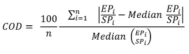
COD = coefficient of dispersion
N = number of properties in the sample
EPi = appraised value of ith property
SPi = sale value of ith property
∑ = summation of all the values in the group
How to Calculate the Coefficient of Dispersion?
After that insane formula, we understand if homeowners want to stay clear of it, but there are reasons why any homeowner would want to use it. If, for example, you’re house was appraised at a value that is higher than you expect, and the same happened to other neighbors, you can figure out if this is a trend in the area to increase taxes or just the increase of the market value in the area.
Example:
John investigated and managed to find the appraised value of 7 properties around him as well as the actual price for those properties.
|
Appraised Value |
Sales Price |
|
359,000 |
370,000 |
|
362,000 |
373,000 |
|
347,000 |
358,000 |
|
329,000 |
340,000 |
|
384,000 |
396,000 |
|
372,000 |
386,000 |
|
395,000 |
396,000 |
Now, John finds out the median appraised value by adding all the appraised values, then dividing it by seven properties ($362,000) and does the same to the median sale price ($373,000). With these values, he can start using the formula.
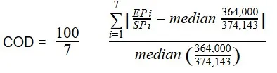
The median appraised value divided by the median sale value is 0.9729.
John returns to his table to discover the EPi/SPi for each property because the ∑ requires him to discover that value independently for each before he subtracts 0.9729 (the median EPi/SPi) from each:
|
Appraised Value |
Sales Price |
EPi/SPi |
|
359,000 |
370,000 |
0.9702 |
|
362,000 |
373,000 |
0.9705 |
|
347,000 |
358,000 |
0.9692 |
|
329,000 |
340,000 |
0.9676 |
|
384,000 |
396,000 |
0.9696 |
|
372,000 |
386,000 |
0.9637 |
|
395,000 |
396,000 |
0.9974 |
With that out of the way, John needs to subtract 0.9729 from each value. Here he considered negative values positive:
|
Appraised Value |
Sales Price |
EPi/SPi |
EPi/SPi-0.9729 |
|
359,000 |
370,000 |
0.9702 |
0.0027 |
|
362,000 |
373,000 |
0.9705 |
0.0024 |
|
347,000 |
358,000 |
0.9692 |
0.0037 |
|
329,000 |
340,000 |
0.9676 |
0.0053 |
|
384,000 |
396,000 |
0.9696 |
0.0033 |
|
372,000 |
386,000 |
0.9637 |
0.0092 |
|
395,000 |
396,000 |
0.9974 |
0.0245 |
Now that he has all the data necessary, John can work the formula:
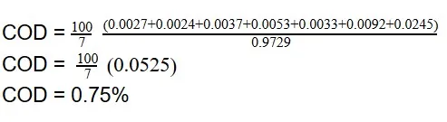
The coefficient of dispersion is a complex formula but the example above tells us that the average difference the houses have from the median of the assessed sales ratio is 0.75%.
Popular Real Estate Terms
Barrel, reservoir, or tank for storing rain runoff. ...
Loose combination of small rocks and pebbles used for a gutter, driveway, landscaping, or roadbed. ...
The American Society of Appraisers, also referred to as ASA, is the largest voluntary membership, a multi-discipline trade association that stands for and promotes its appraiser members. ...
A written agreement between institutional investors to buy or sell ownership shares in mortgages. An institution such as a bank can agree to buy a certain number of shares in a single or ...
Heterogeneous (as opposed to homogenous) means diverse in nature applied to a place or object composed of separate and distinct parts. In other words, heterogeneous describes something that ...
Losses arising from damage to or destruction of property. ...
ADU in real estate is an abbreviation for Accessory Dwelling Units. In everyday discourse, you might have encountered the term under the following nicknames: granny flat, backyard cottage, ...
Deterioration in property resulting from its ordinary use and from the aging process. An examples an apartment building that physically deteriorates over the years. ...
Latin term meaning legal capacity to act on behalf of oneself. ...
Comments for Coefficient Of Dispersion
COD example unclear
Jan 15, 2023 09:18:18Hello. Let us shed some light on this.
Someone wants to find out the appraised value of several properties around them. and the sale price is higher. Then they discover the median appraised value ($362,000). They add all the appraised values of all the properties and divide them by the number of properties. And later does the same with the median sale price ($373,000) The median appraised value divided by the median sale value is around 0.9. Then, they calculate that the average difference between houses and the median is 0.75.
Jan 20, 2023 09:22:24Have a question or comment?
We're here to help.